Cancer survival ML challenge intro

[Apr 2025]

TLDR: I have taken on an ML challenge scored from 0.5 to 1. I am at 0.72 0.75 [as of May] with the top dog sitting at 0.77. More to follow.

Intro: I have taken on an ML challenge¹ to brush up on my ML skills. I picked this challenge as it’s a topic I have no knowledge of and it’s a data structure I have never really worked with before². This post will intro the challenge and explore some data. The challenge is still live so I’m not going to share how exactly I’m making my prediction. That will follow.

The task itself: Participants are tasked with predicting the survival time of cancer patients, specifically those with myeloid leukemia. The details can be found here³, but at a high-level it uses data for ~4500 real cancer patients across 24 treatment centres in France. There are seven clinical metrics given for each patient, and there is a separate dataset detailing the cancer’s mutations, covering ten parameters per mutation, with patients typically having >1 mutation.

On the clinical params: There are six numerical params covering key blood health metrics, and one string param detailing the patient’s cytogenetics.

• Bone marrow blast (%): high equals bad. Indicates proportion of abnormal cells found in bone marrow. Bone marrow is where blood cells are produced.
• White blood cell count (Giga/L)⁴: A healthy range exists. Low WBC production suggests chemo or disease due to marrow damage. High can mean leukemia as it’s a proliferative cancer of blood producing cells, or active infection or inflammatory response.
• Absolute neutrophil count (Giga/L): A healthy range exists. Neutrophils are a white blood cell type key in fighting bacterial infections. Low levels (neutropenia) signal bone marrow suppression or severe infections, while high levels indicate acute infection or inflammation.
• Monocyte count (Giga/L): A healthy range exists. A monocyte is a type of white blood cell that circulates in the bloodstream⁵. They play a role in the immune system by engulfing pathogens and debris and can transform into macrophages or dendritic cells when they migrate into tissues.
• Haemoglobin level (g/dL): A healthy range exists. Haemoglobin is the protein in red blood cells that carries oxygen throughout the body.
• Platelet count (Giga/L): A healthy range exists. Platelets help blood clot, preventing excessive bleeding.

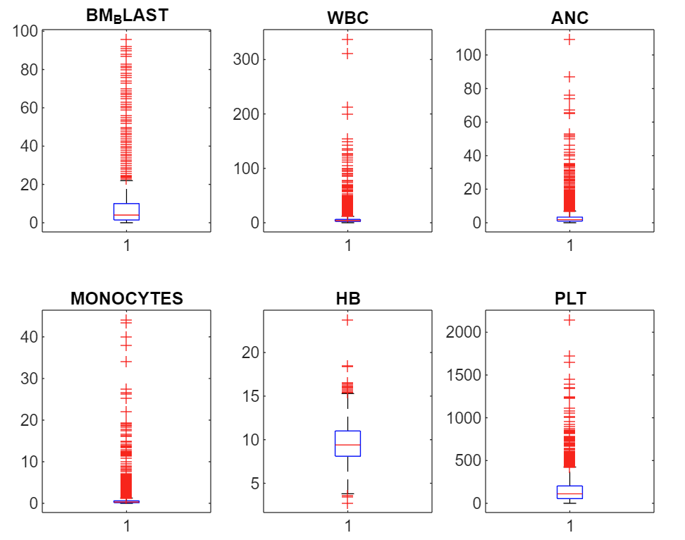
See distributions below. I have cut off some of the outlier data so you can see the distribution shapes more clearly. The green regions are basic healthy ranges.

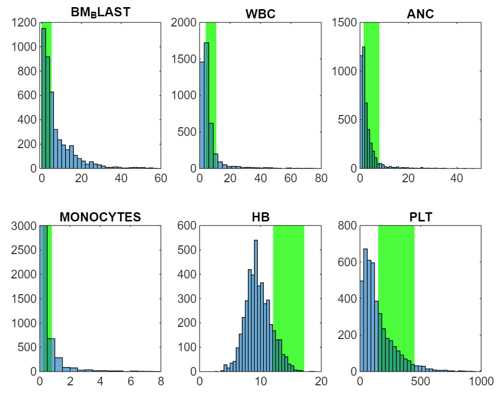
We could use our (assumed) knowledge of what healthy is to create features capturing whether each patient is below, in, or above the healthy range, and by how much. However, the great thing about ML is that this explanatory knowledge is not required and can often be a hindrance. Rather than assume features we should find them statistically where possible.

The last clinical param captures the patient’s cytogenetics in a string, with a typical entry looking like “46,xy,del(20)(q12)[2]/46,xy[18]”. It follows a strict standard⁶, and here it makes sense to extract some features prior to training. There are ~1900 unique cytogenetic categories (prior to proper parsing...), which is far too many to robustly find effects (on ~4500 patients) even if it was our only variable.

On the molecular data: There are only two numeric params in this data, with the rest being categorical like chromosome with 23 possibilities, gene with 143 possibilities, or protein change with 5965. The result is a very sparse dataset. Its also not a complete dataset, with the most frequent protein change being unknown.

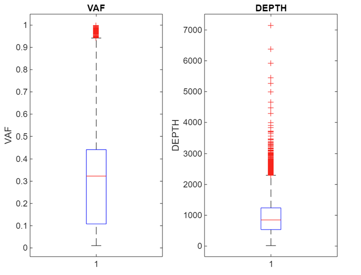
The two numeric params are VAF (Variant Allele Fraction) and depth. VAF represents the proportion of cells carrying the mutation. High is bad. Depth, often called coverage, is the total number of sequencing reads that cover a specific genomic position. A higher depth means more data is available to accurately call a variant and calculate measures like VAF, improving the reliability of the results.

With the molecular data there is also the issue of there being more than one entry per patient. This leaves a tricky chicken and egg problem of needing to compress the features to one row per patient whilst not knowing the most important features, and it takes one row per patient to properly extract the relevant features.

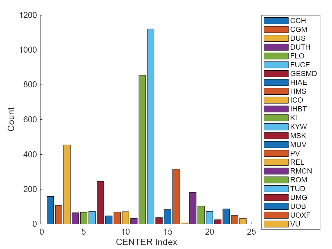
Center bias: One interesting component of the challenge is that the final test set is a completely new treatment center that is not present in the training data. The only way to know before hand if the test center will perform away from average is via center size, which is the only thing we know about it (it is the largest center). Other than that, it could make sense to remove any center effects from the training set…

Survival data and censoring: For each of the patients in the training set we have their survival status at last check up, along with the time to last check-up. We assume that upon death the patient’s status is immediately updated (a safe assumption) meaning there are no deaths reported late. This leaves us with right-censored data for survivors, as we only know how long they have survived so far, not their true time to death.

Benchmarks and performance metric: The key benchmark algo accounts for the right-censoring in the data when fitting the model, and gives a performance metric of 0.66, where 1 is perfect and 0.5 is random. The performance metric itself focuses solely on predicting the patients risk/survival in the correct order by looking at every pair of patients in the dataset. This actually makes sense clinically as its more important to be allocating treatment resources to the most at-risk patient vs having precise bucketing of patient risk where treatment resources would need to be randomly allocated within buckets.

So that’s the challenge fleshed out. I will follow up with my workflow and the technical details in June once the private test set results are up.

Footnotes:

¹ There are a bunch of live and historic challenges here.

² It's not timeseries data, it includes data censoring, and there is a huge amount of categorical data that transforms into a very sparse or low-density distribution.

³ challenge page.

⁴ 1 Giga = 10^9 cells.

⁵ Note that ANC and monocytes are types of WBC. This fact could be used for data cleaning…

⁶ Cyto nomenclature.